Gradient Descent

Whats the right plan to achieve our goals?

  I've come across this story many times in my career... tell me if it sounds familiar to you:  I'm working on a program that has to make a decision about what to do next.  I can evaluate the outcome for whatever decision I make, but I can't predetermine which actions will lead to the best solution.  This is a situation that calls for numerical optimization techniques.  The use of numerical optimization is pervasive throughout computer science.  Artificial intelligence uses it to optimize neural networks.  Engineering tools use it to improve the design of components.  Computer games use it to have the bad guys make decisions that look intelligent.  So how does it work?

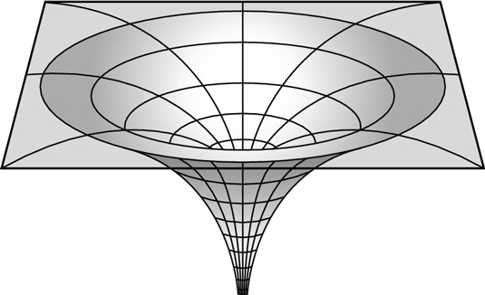Black Hole Gravity Field

  We can start by making a conceptual leap, illustrated by an example.  Suppose you are in a space ship, which you are trying to pilot to the center of a black hole.  You can't see where the black hole is, but you can feel its gravity.  You know that its gravity will get stronger as you get close to the center.  In this example, we can think of the effect of gravity on space as our optimization function.  If we graph that against our position, we get a plot with a nice hole where our black hole sits.  If we had a ball, all we would have to do is set it down on that graph, and let it slide downhill until it reached the center.

Gradient Descent

  This simple strategy is actually the formulation for the gradient descent algorithm.  If at each point, if we know the slope of our function to be optimized, we can just take small steps in the downhill direction.  Eventually, we will reach a point at the bottom of the hill, and that is where we stop.

Gradient Descent Formula

  With this understanding of what we are doing, it is actually very easy to understand the formulation.  Here, F(x) is our function being evaluated, x is our position in the optimization space, gamma is the size of the step willing to take, and n is the step number.  our position at step n+1 can be evaluated as our position at step n plus a small movement in the downhill direction.  When our update fails to sufficiently improve our evaluation, we assume that a local minimum has been reached, and the search is terminated.

Code Design

  From a usability perspective, we want a design flexible for reuse with any arbitrary function to be minimized.  We don't want the user to have to provide a second function describing the gradient of their optimization function.  And we want to allow the user to provide a good guess as a starting point for the optimization.  

        public double Precision { get; set; }
        public double Eps { get; set; }
        public int MaxIterations { get; set; }
        public GradientDescent()
        {
            Precision = 0.001;
            Eps = 0.1;
            MaxIterations = 1000;
        }

  We want to expose a couple parameters that effect the time it takes to reach a solution.  First, we expose the precision we are looking to achieve, typically a very small floating point number.  Next, we expose Eps, which is the step size we take each iteration.  This can be tuned to the scale of your inputs, but typically we still want fairly small steps.  Finally, we expose the maximum number of iterations.  This is a practical measure, as small errors in the gradient can lead to infinite loops near the minimum, while the optimizer bounces back and forth between two positions.  If we get stuck, we rely on the iterations to time out, and a satisfactory answer is returned.

public delegate double Function(List x);
public delegate List Derivative(List x); 

  To represent our optimization functions, the user must implement a function conforming to the first "Function" delegate pattern.  It is designed to map an n-dimensional input vector to a single output metric.  This makes it flexible enough to handle a wide variety of input functions.  We are going to use a second delegate to represent the local derivative, so that we can generate a functor wrapping the input function, generically providing the derivative for easy use.

        public double Distance(List a, List b)
        {
            return Math.Sqrt(a.Zip(b, (i, j) => Math.Pow(i - j, 2.0)).Sum());
        }

  We can recognize an ending connection when the next step is approximately the same location as the current step.  Note that at a local minimum, the gradient of F(x) goes to zero, and thus so does our step length.  We can use the Euclidean distance to measure how much our step has changed, and stop when this metric is sufficiently small.

        public Derivative Gradient(Function f)
        {
            return x => Enumerable.Range(0, x.Count)
                            .Select(i => (f(x.Select((y, j) => j == i ? y + Precision : y).ToList()) -
                                          f(x.Select((y, j) => j == i ? y - Precision : y).ToList()))
                                         / (2*Precision))
                            .ToList();
        }

If you reach back to your calculus class, the definition of the derivative gives us these simple formulations.  I choose to use central differencing, because it is slightly more accurate, but still only requires two function evaluations.

        public List Optimize(Function f, List seed)
        {
            var fPrime = Gradient(f);
            var cnt = 0;
            var x_old = seed.Select(x => x + Eps).ToList();
            var x_new = seed;
            while (Distance(x_new, x_old) > Precision && cnt < MaxIterations)
            {
                x_old = x_new;
                x_new = fPrime(x_old).Zip(x_old, (i, j) => j - Eps*i).ToList();
                cnt++;
            }
            return x_new;
        }

Finally, we have our actual optimization function.  the "seed" variable represents the starting point of the search, and good guesses can dramatically impact the performance of the algorithm.  Also, since we generically defined the Function delegate to take an arbitrary sized vector as input, we need to use the seed to infer a specific size to the inputs of our function.

        [Test]
        public void OptimizerWorks()
        {
            var gd = new GradientDescent();
            var seed = new List {0.0, 0.0};
            var solution = gd.Optimize((data) => { return Math.Pow(data[0] - 2, 2.0) + Math.Pow(data[1] - 4, 2.0); },
                                       seed);

            Assert.AreEqual(solution[0], 2.0, 0.001, "best x found");
            Assert.AreEqual(solution[1], 4.0, 0.001, "best y found");
        }

Now, we have a test showing how to use the module, and voila, a simple C# Gradient Descent module!