probabilistic alpha beta search

Any good chess player can tell you the difference in the styles of someone like Mikhail Tal and Anatoly Karpov.  Tal was known as the magician, someone who sought to guide games into the sharpest possible lines where he could induce mistakes from his opponents, even while taking great risks of his own.  Karpov on the other hand, he was a python.  He'd safely accumulate small advantages, and slowly squeeze his opponent until they cracked.  There styles couldn't be more different, but there results were undeniable; both joined the exclusive club of World Chess Champions.  And yet, neither of these styles are well captured in Computer Chess, who's engines have become the cold assassins of the chess world.  I think capturing the essence of these stylistic differences is a factor that could be used to further improve the results of computer chess engines, and help tailor their response to a given candidates strengths and weaknesses, without compromising quality.  What is the missing factor?  Quantification of risk.

Figure 1: Game tree with mimimax highlighted in red, and prospective better path in green

What does it mean to include "risk" in a turn based two player zero sum game?  Consider Figure 1, which highlights the typical  minimax approach to game trees in red.  Each player has competing goals, Max is looking to choose a path that maximizes his score, thus picking the maximum nodes in the next level, while Min is trying to minimize the score on his turn.  Scores are bubbled up from the bottom.  We see from this perspective, Max's optimal choice would be to pick the left branch, because given optimal play from Min, the score of 1.2 produces a slightly superior position.  If the scores were perfect, indeed this analysis would be correct, and risk would be completely mitigated.

The reality in games where the search depth rarely allows one to reach terminal nodes is that we use a heuristic as a proxy for the true score.  When the frontier node is finally reached, we repeat the process of creating a tree to search, bubbling up a new score that serves as a better estimation of the actual value of the position at that node.  This means there is a variance in the heuristic that must be considered when choosing our path through the tree.  When we eventually reach a pre-frontier node, we will have reached the last responsible moment from which we can change our decision.  The score of pre-frontier nodes as viewed from the root must then be some combination that accounts for the likelihood that the proxy score for any frontier node has improved by the time we reach the pre-frontier level.

Consider node A vs node B.  If we were to reach node A and then discover that our heuristic evaluation overestimated the score of the child node valued 1.2, we have left ourselves without a viable alternative, as the variance in our heuristic score is unlikely to overcome the 6.2 point gap we predicted in the alternative branch.  If the true score of the best choice at node A was -1.0, we would have no recourse but to continue down that path.  Node B, on the other hand, provides two choices of similar value.  If we were to reach Node B and discover that our 1.1 option actually produced a score of -1.0, we would still have a viable alternative in the 1.0 node.  Minimax fails to capture this characteristic.

Now consider nodes C and D.  From the prospective of Max, we again recognize that Min's options are restricted at node C due to the large difference between the first and second best nodes.  It is not likely that the variance in the 4.0 node will overcome the gap in scores, which means that a miss-evaluation of the frontier node in Max's favor cannot be mitigated by a second choice from Min.  Node D however does provide that alternative, in the similar score of the 1.3 node.

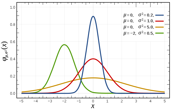Figure 2: Normal Distribution

What we are interested in is creating a probability distribution that models the difference between the quiescence score of a frontier node (such as the 1.2 valued node in Figure 1), and the score of that same node if it were fully evaluated one ply deeper than the root (such as the position of node D in Figure 1).  That is to say, we need to understand how much our heuristic evaluation will vary between the time when we first encounter a node in the search tree, and our last chance to change our mind.  A normal distribution (see Figure 2) may be an appropriate model for a good heuristic, where the x-axis represents the score, and the y-axis represents the probability.  This model can be fitted empirically ahead of time, sampling quiescence and max depth evaluation pairs.

Figure 3: Cumulative Distribution Function

Integration of the normal distribution leads to the cumulative distribution function, pictured in Figure 3.  This function can be used to describe the probability that a random draw from the normal distribution will be less than X.  For example, a random draw from the distribution represented by the green curve in Figure 3 will be less than -2.5 20% of the time, if we trace 0.2 on the y-axis to the intersection.  That means with 80% certainty, that distribution is greater than -2.5.

Figure 4: Three choices represented by three cumulative distribution functions

Now consider the situation in Figure 4, where our search has reached node A (a pre-frontier node), in the context of a much larger search.  Nodes B, C, and D are individually represented by the cumulative distribution functions F1, F2, and F3.  We can hedge against the risk of any single node by combining the three cumulative distribution functions to get a single distribution, one which represents the probability of the score of the best of these three alternatives as determined by a full depth search rooted at node A.

Equation 1: Recursively defined CDF accumulating all move alternatives

Equation 1 expresses a combined cumulative probability distribution recursively, where Fi represents CDF for the ith alternative move choice.  Here, we can say at any point that the probability that a random draw from a distribution is at least as great as X is equal to the probability that Fi is greater than X, plus the probability that Fi is less than X times the probability of the combination of the remaining alternatives is greater than X.  A concrete example can be again taken from Figure 3.  Consider the blue, red, and orange distributions, each with its mean at 0 (ie: F1(0) = F2(0) = F3(0) = 0.5), and assume those represent the probability distributions for Figure 4.  Each by itself has a 50% chance of scoring higher than 0.  Combining those into Equation 1 and expanding the probability around 0, we find that we have an 87.5 percent chance of scoring better than zero.  This completely upends our understanding of the score at node A in Figure 4.

We can incorporate this probabilistic model into the existing framework of Alpha Beta Search.  Our search algorithm is initialized with a confidence parameter denoting the risk we are willing to take in selection of our next move.  I would expect that requiring a high confidence (95%) would produce strategically sound games with little risk, as in the style of Karpov.  Requiring low confidence (5%) would result in riskier search paths, but higher rewards, as in the style of Tal.

At every terminal node, the Quiesce function instead returns the cumulative probability function mapping to the score produced by our heuristic evaluation.  Every non-terminal node produces a combined CDF using the methodology described by Equation 1.  Bounds are set by evaluating a CDF at the prescribed confidence level, giving us a fixed expected value to compare against as Beta.  Then, when a child is iterating through its move choices, it updates the probability that one of its subnodes will be greater than Beta.  If the probability is greater than our prescribed confidence, we can do a beta cutoff.  One of the nice consequences of this strategy is that as the variance of our heuristic evaluation drops to 0, the search converges back to a normal alpha beta search.

References to other related approaches:
B* Search
ProbCut Pruning
Conspiracy Search

Similar approaches in the literature:
An optimal game tree propagation for imperfect players